visionCATS Guide

General Introduction

The visionCATS concept: HPTLC made easy!

visionCATS is CAMAG’s current HPTLC software. It stands for ease of use and intuitive simplicity. The software organises the workflow of HPTLC and controls all involved CAMAG instruments and the CAMAG® HPTLC PRO. The easy-to-navigate user interface guides effectively through the chromatographic process – from analysis definition to analysis reporting.

As state-of-the-art software, visionCATS is based on a client-server system offering enormous flexibility to the number of instruments and users that are working together, enabling access to the same data for all members of a work group. The sample-oriented approach allows for creating virtual plates with tracks originating from different plates, for example, batch-to-batch comparison or long-term stability testing. With visionCATS relevant samples can be located easier and faster than ever: a powerful search tool and a file explorer that includes extended preview functionalities enable highly comfortable searches for samples, methods, and analysis files.

The default settings implemented in the software were chosen according to the general chapters of the USP (chapter ‹203›) and the Ph. Eur. (2.8.25). This enables analysts, who work in a cGMP regulated environment, to run standardized HPTLC without the need for modifications in the software settings. In addition, visionCATS provides a Method Library with procedures that are in full compliance with chapter ‹203› (see Working with methods from the Method Library). All HPTLC methods of the USP Dietary Supplement Compendium (DSC 2015) are included. Other library methods of identification originate from the European Pharmacopoeia and the HPTLC Association. Methods developed by CAMAG are in the library as well.

visionCATS was developed for working in routine labs with validated methods. The primary focus is on following a standardized methodology (supported by the default settings according to the general chapters of the pharmacopoeias) to obtain reproducible and reliable analytical results. Data (digital images /scan data) should be qualified by a System Suitability Test (SST). visionCATS supports compliance with cGMP/GLP and 21 CFR Part 11.

Key features

• Supports qualitative and quantitative HPTLC Analysis

visionCATS organizes the workflow, controls the involved CAMAG instruments, and manages data.

• Comparison Viewer

The sample-oriented approach allows for creating virtual plates from tracks originating from different plates. In the Comparison Viewer samples can be compared on the same screen side by side using selected racks of images (HPTLC fingerprints) or peak profiles of the tracks (generated from images and/or or obtained by scanning densitometry). Furthermore UV spectra of individual substances/peaks can be compared.

• Image enhancement tools

visionCATS supports low-noise, high-dynamic range imaging (HDRI) and includes a comprehensive set of Image Enhancement Tools (Data view).

• Method Library

visionCATS provides a free of charge HPTLC Method Library for licensed users (see Working with methods from the Method Library)

• Flexible Reporting

visionCATS contains a fully configurable reporting system for analysis and comparison files (see Report Settings)

Benefits

• Enhanced usability

  • Focus on usability and modern appearance

  • One-click solution with semi-automatic settings

  • 3 levels for the user interface (easy, medium and expert). All levels are in reach of one mouse click.

• Guidance on workflow

  • While executing a method, the user receives information about the status of process, required actions, and the subsequent steps of the analysis.

  • The parameters for a step can still be edited/modified before the step is executed.

• State-of-the-art Architecture

  • visionCATS features a client/server architecture, enabling scalability from a single workstation to a multi-user lab network

  • Easily extendable

  • Easy to install (plug & play) and to service

• Compliance

  • User management (different contents/rights, passwords) for data security

  • Backup (with schedule assistant) for data safety

  • 21 CFR Part 11 (System logger, E-Signature, options related to deletion, motivated change management; for further information see online help at: 21CFR Part 11 compliance

  • Qualification (IQ/OQ)

  • System Suitability Test (based on RF values of marker compounds) to check and ensure that the analysis was performed appropriately. The test is passed when the detected peaks are positioned within the range established during method development.

Getting Started

Main window

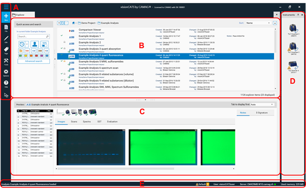
Elements of the Main window:

A Main Toolbar

B Explorer and search window shows available projects / files (and their status)

C Preview window (shows preview of a selected file)

D Optional: Instruments window (shows all installed instruments and their connection status)

E System Status Bar

visionCATS was developed for routine work. Users work in “project folders”. In each folder, a method file is created first, which is based on a validated method documents and the standard operating procedure of the lab (e.g. template Ph. Eur. 2.8.25). All analyses performed with the method are typically stored in the same project folder. Comparison files generated from the analyses belong here as well. To create a new general method template, a new method, or a comparison file an existing folder needs to be selected from the explorer or an additional one created (New folder): Select New / New folder from the main toolbar.

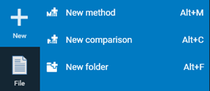
Then in the open folder a new method/comparison can be created (selection at the New menu). For creating own methods go to Creating a new method.

Working with method templates

visionCATS supports routine work according to the general chapters on HPTLC of the USP and Ph. Eur. For this, different method templates are provided. On CAMAG’s website, method templates are available for download. Go to Downloads and download the ZIP-folder “Method Templates”.

The downloaded method template(s) can be imported into the visionCATS database, selecting/creating an appropriate folder, e.g. templates.

The templates include HPTLC standard parameters for all steps of qualitative analyses (no scanning densitometry). To create a method for an individual project based on the template, right click the template and select copy to or press Ctrl+Shift+C and then save the method with the name of the selected project. Next, open the new method and add information about SST, developing solvent (mobile phase) and derivatization and change any parameters that are not according to the standard template. After saving the new method file is ready to use.

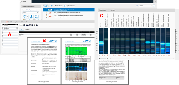
Working with methods from the Method Library

The CAMAG Method Library is a repository of methods that can be downloaded directly a visionCATS installation. Each method package includes three files:

• An instrument method (A) ready to use in visionCATS in two versions (one for Linomat 5 and another one for the ATS 4)

• A method document (B) in a form (e.g. docx) which may serve as an SOP. This file contains a description of the System Suitability Test (SST) and acceptance criteria for passing samples

• An Image Comparison file (C) with reference images against which each analyzed sample can be compared and evaluated,based on acceptance criteria specified in the method document

For download of methods from the library and method transfer validation, see Method transfer.

Method transfer

Downloading a method from the Method Library

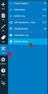
To download a method, click Tools on the Main Toolbar and select Method Library.

The overview page of the Method Library will open.

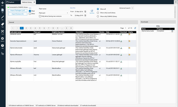
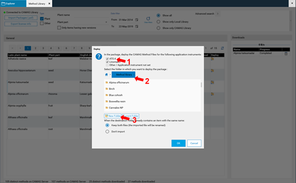
CAMAG continually adds new methods. Please note that new methods generated with the most recent version of visionCATS are not compatible with previous visionCATS versions. To have access to all methods an update to the latest version of visionCATS is required. The selected method is downloaded by clicking on the arrow button (1). The download progress is shown at (2). When download has finished the method can be imported to the database by clicking on (3).

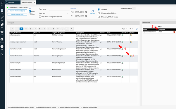
In the next step the suitable version of the instrument method (ATS 4, Linomat 5, or both) are selected at (1), then the destination folder is selected at (2), or if a new folder is created at (3).

Note: For a direct access to the Method Library an internet connection is needed. The companies’ firewall needs to allow access to Method Library. visionCATS communicates via Port 10501 (default). For lab PCs with no Internet access methods can be downloaded with the Standalone Downloader as PXF files and later imported using the Import Packages (.pxf) button. You can find the Standalone Downloader installer in the visionCATS server’s installation folder (the default installer file is located at C:/Program Files (x86)/CAMAG/visionCATS/MethodCollectionMainInstaller.exe). When opening the Standalone Downloader for the first time, you will be prompted to import your license file. The Standalone Downloader has a user interface and functionalities similar to the Method Library tool of visionCATS, except that it downloads the files to the user-definable destination folder.

Performing a method transfer validation

Method transfer to your lab is very simple: transfer validation stipulates that the SST (System Suitability Test) must pass! After downloading and importing a method from the Method Library, you can access the imported files from the Explorer window. Each method includes a method document that describes the entire procedure and the RF values for the SST. Execute the method as described and the check the SST according to Section 9. Unless otherwise stated in the method document CAMAG recommends as general acceptance criterion that the 𝑅ꜰ should not vary more than ∆0.05.

Check out our case study Identification of fixed oils by HPTLC to see how method transfer is done: Identification of Fixed Oils

Creating a new method

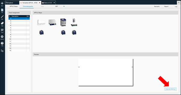
To create a new method or method template from scratch, a folder needs to be selected or an additional one created (New folder) from the main toolbar (selection at the New menu).

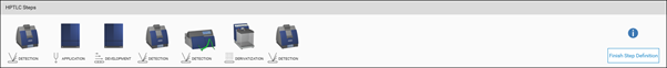
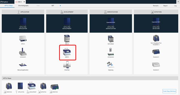
Then in the open folder a new method can be created (selection at the New). After entering the name (usually the same as the project folder) click Ok. A new window open, where the required steps can be selected by clicking on the instrument icons. The steps will be added to the bottom area and (later) executed in the order from left to right. Steps can be deleted if needed or rearranged in the bottom area by dragging/dropping them.

With a click on Finish Step Definition the settings window will open

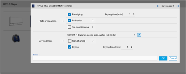
Use the device icons to change settings like solvent type for application, SST requirements, developing solvent (mobile phase), etc. All settings that are fix for the respective method must be entered. Default setting for each step including the plate layout are in compliance with ‹203› / 2.8.25.

By clicking Execute Method the analysis can be performed.

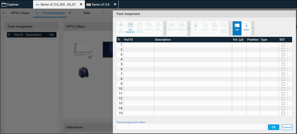
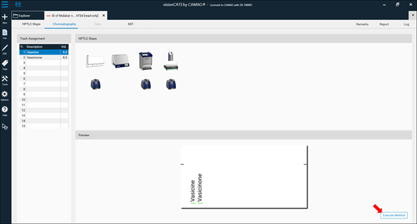
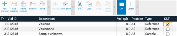
For each analysis, the Track Assignment table is opened first by clicking it. Enter for each sample and standard (reference) a unique Vial ID, enter the application volume, select the rack position (for HPTLC PRO Module APPLICATION and ATS 4), select type (sample or reference) and tick tracks used for the SST. In the Description additional information on the sample/reference can be added.

After clicking OK, visionCATS will guide you through the different process steps.

Creating a qualitative method (e.g. identification of a herbal drug)

All process steps are selected as descripted in the method document. It is recommended to start with a Documentation (TLC Visualizer) step. This will be recognized by the software as “Clean Plate” image(s) and subtracted automatically from the image captured after development.

A typical scenario could be:

First capture an image of the empty plate, then apply the samples/references, develop the plate, capture an image of the developed plate, derivatize the plate, and capture an image of the derivatized plate.

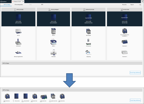
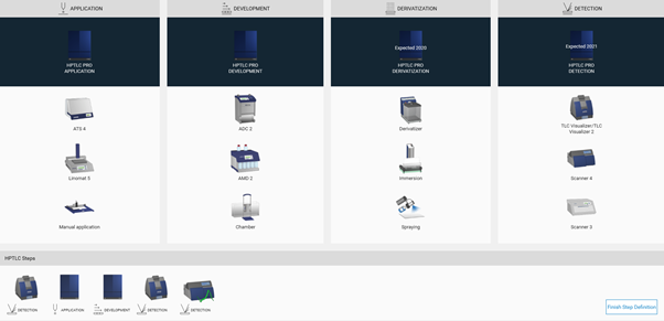
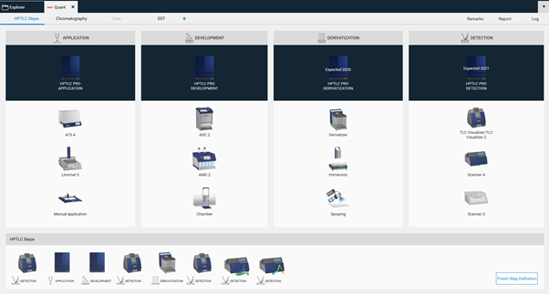
The related HPTLC process includes those steps:

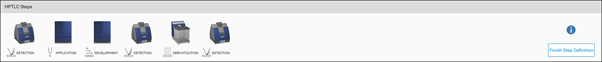
The sequence and number of process steps can vary depending on the method. Each step can be also be performed multiple times (e.g. an image prior to and after derivatization or with different capture settings, different ATS 4 for different dosage speeds for application of samples prepared with different solvents, two or more derivatizations).

Note: visionCATS supports different options for each process step. Samples can be applied either by HPTLC PRO Module APPLICATION, ATS 4 (Automatic TLC Sampler), by Linomat 5 (semi-automatic TLC Sampler) or manual with capillaries (Nanomat). Development can either be performed isocratic with the HPTLC PRO Module DEVELOPMENT, ADC 2 (Automatic Developing Chamber), by gradient with AMD 2 (Automated Multiple Development), or manual with a tank (Twin Trough Chamber, Flat Bottom Chamber, Horizontal Developing Chamber with different dimensions). Derivatization can be done by immersion (with the Chromatogram Immersion Device), by automated spraying (with the Derivatizer) or by manual spraying, Data Acquisition can be done with the documentation system (TLC Visualizer/TLC Visualizer 2) and by scanning densitometry (TLC Scanner 3/TLC Scanner 4).

Creating a quantitative method

For quantitative methods two different options are available for Data acquisition. Either peak profiles can be generated from captured images or densitograms can be recorded with the TLC Scanner.

A typical scenario could be

First capture an image of the empty plate, then apply the samples/references, develop the plate, capture an image of the developed plate, scan the developed plate in absorption and/or fluorescence mode, derivatize the plate, and capture an image of the derivatized plate.

The sequence and number of process steps can vary depending on the method. Each step can be performed multiple times (e.g. a scanner step prior to and after derivatization).

Performing an analysis

The visionCATS workflow is based on instrument methods (either derived from method templates, provided by CAMAG, or created from scratch). A method is required before an analysis can be performed. Between different methods, HPTLC is a very flexible technique. For high reproducibility of analytical results flexibility must be limited within a method.

By clicking Execute Method a window opens and the name of the respective analysis file can be entered. By default the name is created with the method name combined with date and time.

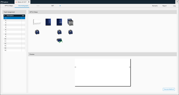
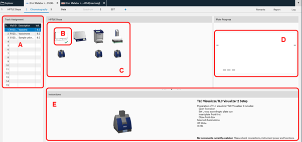
After confirming the name by clicking OK the Chromatography tab of the analysis file will open. In there, all settings and parameters can still be edited (not recommended). For routine work only information in the Track Assignment table (A) must be entered after clicking it. More information on the Track Assignement table is available at:

Track Assignment

visionCATS is guiding through the analysis. In (B) plate layout parameters could still be edited (this should rather be done in the method). In (C) the entire HPTLC process is displayed. All steps can still be edited as long as they have not been executed). Completed steps are marked with a green arrow (B). In (D) a preview of the plate layout is shown. When executing a step, progression and instrument status are also displayed in this area. (E) provides instructions for the analyst, available instruments, and displays generated data during the execution of a step.

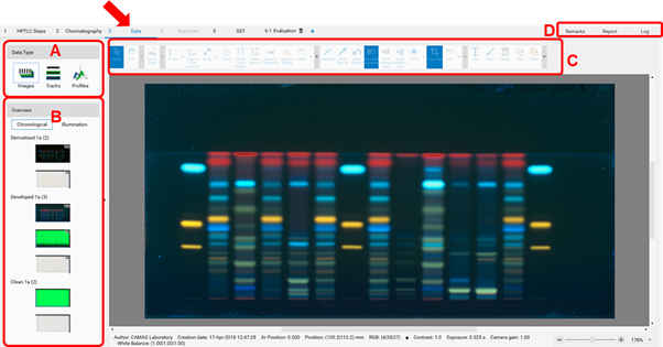
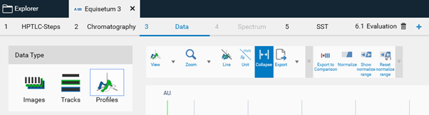
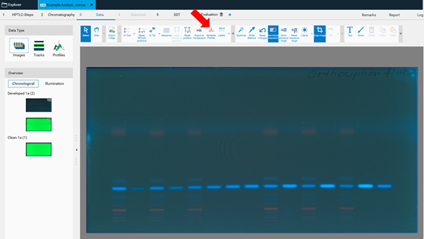
Data view

After all steps of an analysis have been executed, the Data View will open. The last captured image will be displayed. (A) allows to switch between three different views: Images (images of the entire plate), Tracks (track-oriented view), and Profiles (image profiles and/or densitograms). (B) displays the sequence of all captured images within this analysis. By clicking either the entire plate is shown in the respective detection mode. (C) is the Data View Toolbar, containing general tools, 𝑅ꜰ and track tools, and image enhancement tools. More information on the Data View Toolbar at:

DataView Toolbar

In (D) Remarks can be added to the analysis file (e.g. import an image of MS data obtained by HPTLC-MS) that will be displayed in the report and a “Report” can be generated (per default a full report of the whole analysis will be generated, including all settings, run time, results, etc.). Custom report templates can be saved and set as default. More information at:

Reports Configuration

By clicking Log (D) (requires option 21 CFR Part 11) the Analysis log file will be displayed.

Tools

The Toolbar in the Data view contains all tools for image editing and image data processing (general tools (A), 𝑅ꜰ tool and select tracks for comparison (B), image enhancement tools (C), annotations (D)).

All icons are explained at: DataView Toolbar

The most relevant icons are in section (B) and (C):

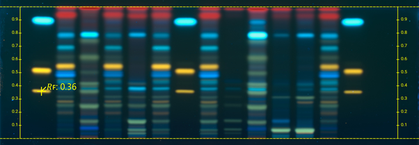
(B): 𝑅ꜰ Tool displays lines at 𝑅ꜰ 0 and 𝑅ꜰ 1 (region of interest)

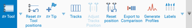
𝑅ꜰ Tip adds an 𝑅ꜰ value to a zone of interest

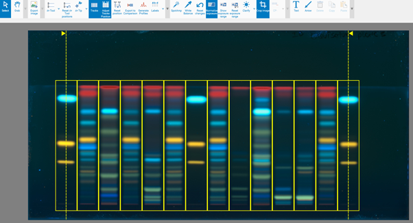
Tracks allows selecting single or multiple tracks for image comparison (and together with Adjust Tracks Position to optimize the track position and width, if needed).

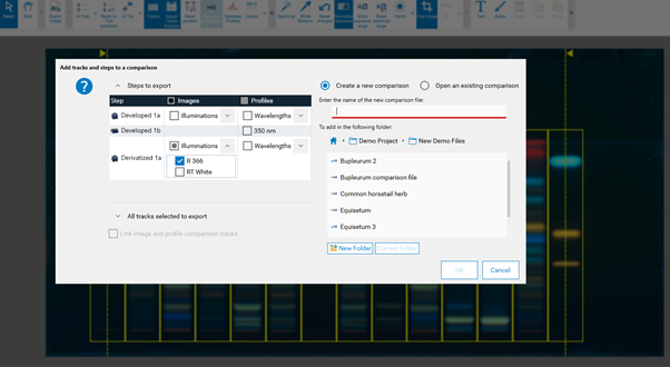
By clicking Export for Comparison a new window opens. File name, tracks, and detection modes (images and profiles) for a Comparison file can be selected. Further information is available in Section 14.

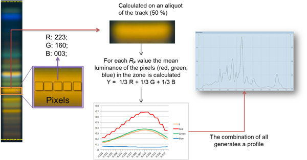
By clicking Generate Profile image profile are generated (for each (pixel) line of the track visionCATS calculates the luminance from detected RGB values). Plotting the luminance as a function of 𝑅ꜰ values generates peak profiles, which can be used for image-based quantitative evaluations. Data are accessible in the track and profile view, and in an evaluation tab.

(C): Image Enhancement tools

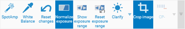
SpotAmp increases the contrast of the zones. After selecting the SpotAmp tool click the background once or up to four times (maximum contrast 4.0). Original data are displayed after clicking Reset changes.

White Balance allows to re-define “what is white” by clicking the part of the captured image with a white background.

Normalize Exposure allows a normalization of the entire plate to one reference track. The default is set on track 1 and can be changed in the general settings. This feature is active for High Dynamic Range Images (HDRI) captured under UV 366 nm (sequence of images with different exposure times summarized in one). By clicking Show exposure range the selected track for normalization and allows a manual change are displayed. This feature was implemented for comparing samples originating from different plates in fluorescence mode.

Clarify virtually changes the illumination setting after capturing to make weak zones better visible (for HDR images).

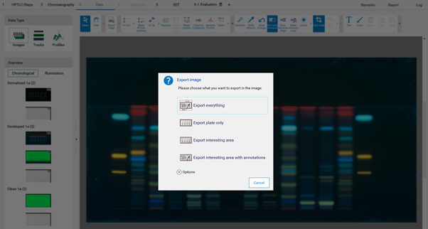
Export of Images

For export of images different options are available. Access the window Export Image by clicking the icon at the tool bar or by right mouse-click on the captured image. Images can be exported with or without annotations to a local disk or copied to clipboard for copy-paste to another file (e.g. a Word file).

Working with SST

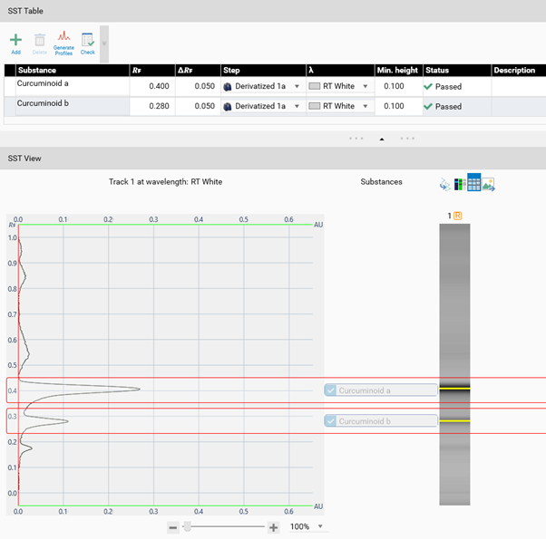
The SST (System Suitability Test) is a test for assessing quality and reproducibility of the chromatographic system. CAMAG has implemented an SST according to the recommendations of the HPTLC Association. Methods from the HPTLC Association feature a set of standards with defined 𝑅ꜰ positions. For instrument methods from the visionCATS Method Library the Δ𝑅ꜰ was set to 0.05. This is a recommendation for analyses performed on different days or in different laboratories. Other criteria can be defined.

For the SST a tick on the respective track(s) in the Track Assignment table (Chromatography tab) is required.

After performing an analysis the SST can be validated in the SST tab.

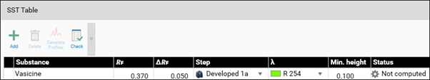
Example: In the SST tab, the acceptance criteria for the SST are added (pre-set in the method template or set in the performed analysis). Then the detection mode(s) (wavelength(s)) for validating the SST is/are selected. For SST on images a profile must first be generated (Generate Profiles). Then click Check for computed evaluation (maximum of a peak within the window will be detected if AU is larger than 0.1) and indicated by a green (passed) or red (failed) arrow.

Note: It is possible to mark an SST definition as passed manually via the check box on the banner.

Scanning Densitometry

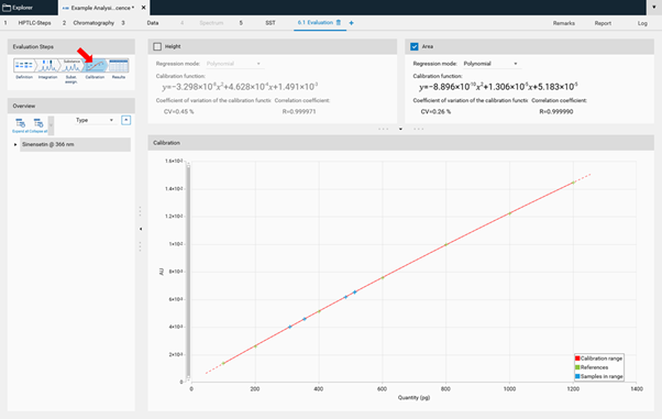
visionCATS controls the TLC Scanner 3 and TLC Scanner 4. Scanning densitometry generates spectrally selective quantitative responses for the individual tracks of the HPTLC plate as “Peak profiles from densitometry” (PPD). Several scanning steps (e.g. after development and/or after derivatization) can be programmed (single wavelength, multiple wavelengths and measurements in absorbance and/or fluorescence mode). For any detected peak on the plate, a UV-VIS spectrum can be recorded. For evaluation of the data, visionCATS provides five different calibration functions (e.g. linear and polynomial). Based on spectral data, peak purity can be determined.

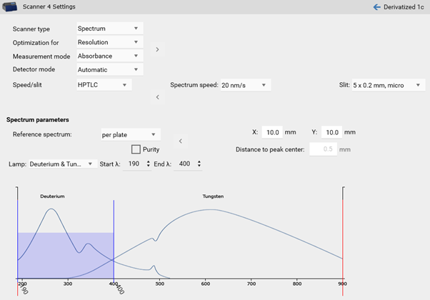
The optical system

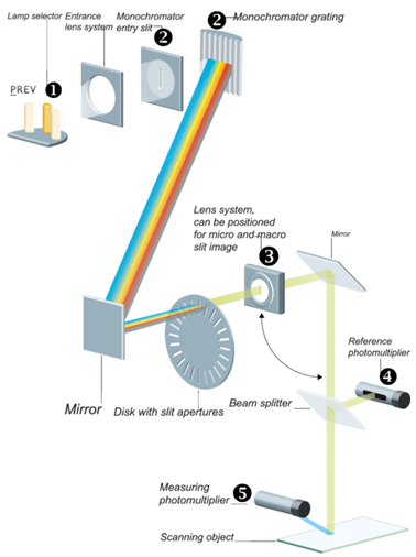
Any of the three light sources, high-pressure mercury lamp, deuterium lamp, or halogen-tungsten lamp can be positioned in the light path by a motor drive. (1) (Further information can be found in the TLC Scanner Manual)

Single-wavelength scan

For a single-wavelength scan, a scanner step is added to the HPTLC process in the method template.

By clicking Finish Step Definition, you will get to the Chromatography tab. Clicking the Scanner icon opens the Scanner settings.

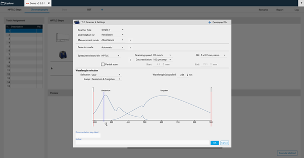
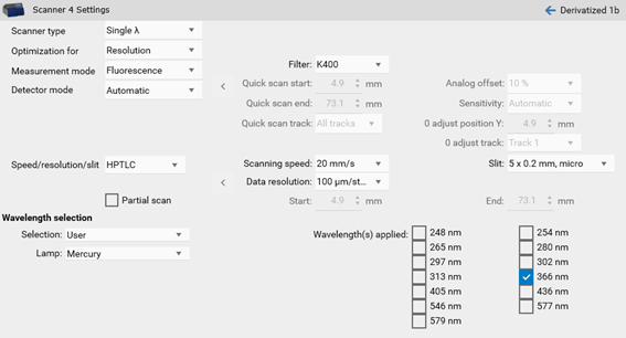
There, Scanner type (Scanning mode), Measurement mode and Lamps can be chosen. Default is set to single-wavelength scan in absorbance at 254 nm. If another value is entered, e.g. above 400 nm, then the firmware will switch on the lamp for this range (deuterium lamp for UV range and tungsten for VIS range). If you select fluorescence mode, then you can select the wavelength for excitation (either deuterium/tungsten or selection of a spectral line of the mercury lamp). For fluorescence detections between different cut-off filters can be chosen, e.g. for excitation with 366 nm the filter K400 is well suited for filtering the light to be detected (only light above 400 nm can pass the filter).

In certain cases, changes to the default settings for scanning speed, data resolution and slit size makes sense. The wider the slit, the higher the light intensity while resolution of peaks is reduced. Especially for small peaks data resolution set to 25 µm will lead to better results.

Multi-wavelength scan

If multiple analytes in the same analysis absorb at different wavelengths or if a subsequent measurement in fluorescence and absorbance is needed, a multi-wavelength scan can be performed.

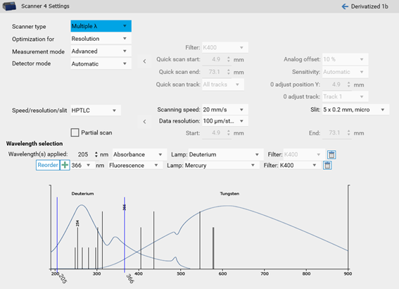
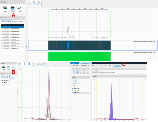
Image profiles

With the Visualizer Ultimate Package Peak Profiles from images (PPI) can be obtained with a mouse-click. The software calculates for each track the resulting luminance (in the middle of the track) and plots it as a function of the 𝑅ꜰ value.

To generate PPI, just click the icon in the Data view toolbar.

PPI are available in the Tracks view (A), in the Profiles view (B), and in the evaluation tab ((C) for quantitative evaluation).

Evaluation

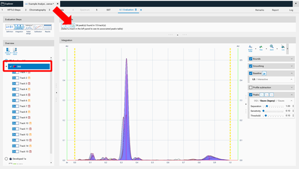
After all steps of an analysis have been executed, an evaluation tab can be added (click plus to open an evaluation tab). Up to five different evaluations can be performed for each analysis file. visionCATS supports different user levels. In Basics of quantitative evaluation in visionCATS the Easy mode is described.

Basics of quantitative evaluation in visionCATS

visionCATS guides you through the evaluation process:

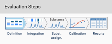
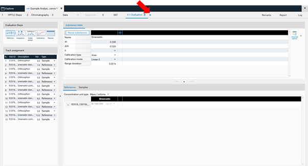
In Definition the substances to be analyzed and their concentration in the reference vials are defined. The quantity applied of each reference will be calculated from the application volume and the defined concentration. At (A) (red arrow) substances can be added and named. At (B) the concentration of the reference solution(s) is (/are) entered.

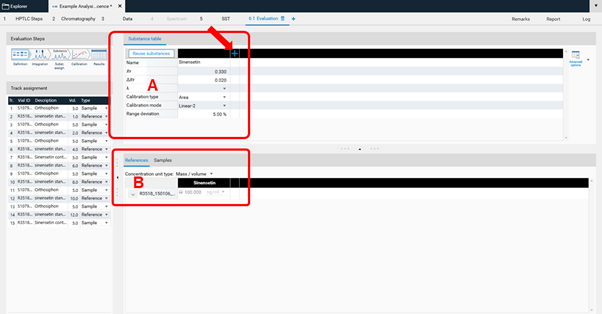
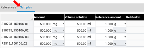
Use the tab Samples to define the sample reference amounts.

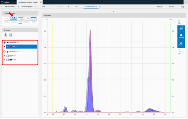
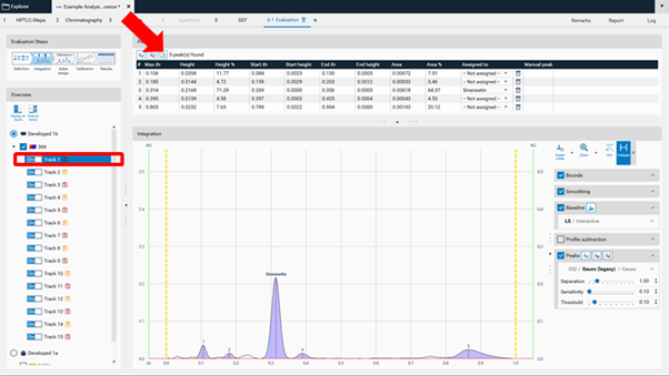
Continue with the next step Integration. The profiles (PPD or PPI) are displayed here. On the left side, different detection modes can be selected.

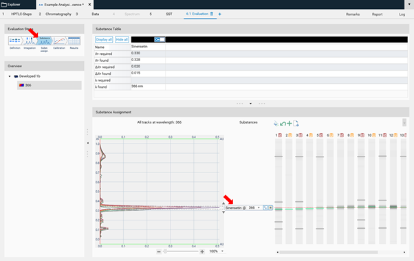
In Easy mode, you can directly continue with the next step Substance Assignment and position the substances at the proper 𝑅ꜰ (moving each substance name to the expected 𝑅ꜰ position).

In the next step, Calibration the best fitting regression mode is selected (and applied for evaluation via peak height or area).

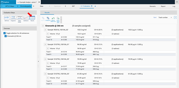
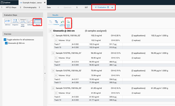
In the final step Results, a summary of the quantified amounts/concentrations of each substance in the sample(s) is shown.

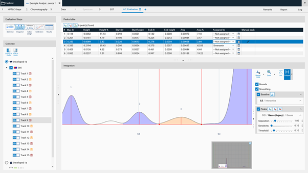
Manual mode

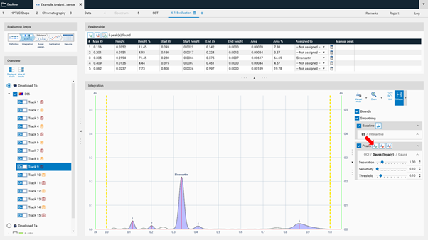
In the Integration step, you can select one of three user levels. Default is the Easy mode. On the right hand side a switch to Manual mode can be done. In the Manual mode, advanced baseline and peak detection features are enabled, and the peak table is shown. Use this mode for manual peak integration.

To add a peak select the Add manually a peak icon.

Ctrl + Mouse-scroll allows zooming-in.

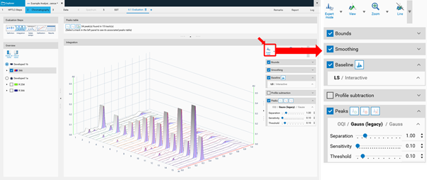
Expert mode

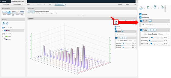
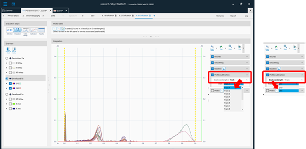
In the Integration step you can select one from three user levels. Default is the Easy mode. If Expert mode is selected, all available features are accessible. Use this mode to configure advanced features such as smoothing parameters, (blank) track subtraction and dual wavelength subtraction.

Bounds

Bounds limit the evaluated data to those between the start and end bound (in RF unit). Clip outside will hide data outside the bounds.

Smoothing

Profile raw data usually have some noise, which can adversely affect the peak detection. Smoothing can remove this noise. There are three smoothing algorithms available: Savitzky Golay (SG, which is the default), Moving average (MA), Gauss (newly implemented for visionCATS). For each algorithm, a window or width can be adjusted to specify the degree of noise filtered.

Baseline

By default background correction is done with the slowest slope algorithm (automatic baseline detection, works on most data). Interactive allows manually adding baseline segments for background correction. To display the detected baseline use the button Display Baseline.

Profile Subtraction

Dual Wavelength: select a base wavelength in the combo box. For each track PPD of the base wavelength will be subtracted from the PPD(s) of the other wavelength(s) selected.

Track: select a base track in the combo box. The PPD of this (blank) track will be subtracted from the PPD of other tracks.

Peaks

For peak detection two algorithms are available: Optional Quadratic Interpolation (OQI) and Gauss (default). For both peak detection algorithms the Separation, Sensitivity and Threshold parameters.

Peak table export

In Manual and Expert modes the peak table can be exported of either a single track or of all tracks as csv files (comma separated values) for evaluation in Excel or other software.

Related substances

The feature Related substances allows determining the impurities within a sample (e.g. in an active pharmaceutical ingredient). For calculating the percentage of an impurity (impurities) a calibration curve of the main substance is generated. In the Definitions step of the Evaluation on the right hand side (A) Advanced Options are available. If Related substances is selected, the drop down list in (B) allows assigning the main and the related substance(s). There are three modes for evaluation: classic, by dilution (fixed volume), and by volume (fixed concentration). The classic mode (default mode) calculates the quantity of impurity/impurities based on the concentration of the main substance. In By dilution and By volume mode one track is defined as reference concentration/application. This can be defined in the Related substances parameters. The result is then calculated in % impurity. Different calibration levels of the main substance can be generated by applying individual standards (same volume/by dilution) or a single standard (different volumes). For this feature, two example files are available for download (Example Analysis 8 related substances (volume) & Example Analysis 9 related substances (dilution) in the provided zip-folder: Downloads ).

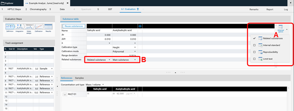
Via the advanced mode (A) the Related substances feature can be accessed. Then in (B) Main and Related substance(s) are selected.

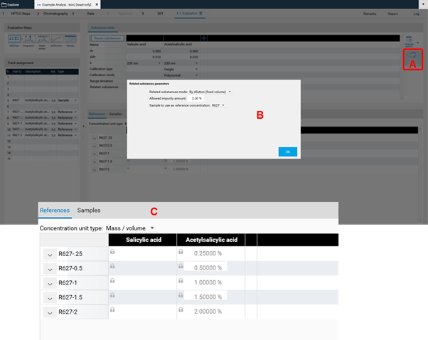
At (A) the Related substances parameters can be accessed. Default is the classic mode. For the Related substances by dilution one sample track is defined as reference concentration (B). In (C) the concentration of the individual standard solutions is entered.

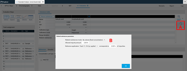
At (A) the Related substances parameters can be accessed. Default is the classic mode. For the Related substances by volume one sample track is defined as reference application (B).

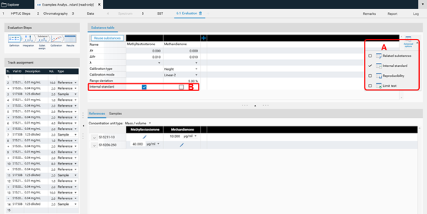
Internal standard

The feature Internal standard may increase the accuracy of the analytical result. By addition of an internal standard to all samples and standards the variations in the sample preparation (different extraction yields) and errors in the measurement chain are reduced/corrected. In the Definitions step of the Evaluation on the right hand side (A) Advanced Options are available. If Internal Standard is selected, in (B) with a tick, the analyte used as internal standard is selected. The Example Analysis 7 Internal Standard” (download zip-folder at: Downloads) provides an example.

Reproducibility

The feature Reproducibility evaluates the deviation of the peaks height/area of a certain substance applied on several tracks. For each substance, the reproducibility test calculates: * the average (height or area) * the coefficient of variation (CV) * the deviation of each value from the average.

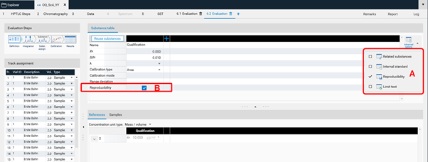
At (A) the Reproducibility feature can be accessed. Use the check box at (B).

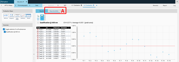
In the Results tab, the Reproducibility results are displayed in a separate tab (A).

Limit test

The feature Limit test determines whether the quantity or concentration of a substance in one or more samples is above or below a specified limit. The Limit test is a fail/pass check for each individual sample track.

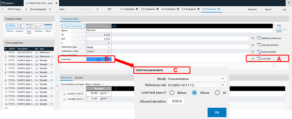
At (A) the Limit test feature can be accessed. Use the check box at (B). Set the criteria at (C).

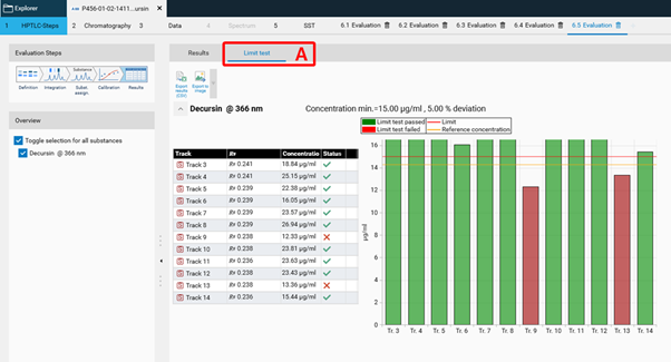
In the Results tab, the Limit test results are displayed in a separate tab (A).

Export results

The results table can be export as .csv file for e.g. further evaluation in Excel.

Export graphs

All graphs (calibration curves, spectra, limit test results, reproducibility results) can be exported by a right mouse click. The graphs can be exported with different resolution and saved to a destination folder or to clipboard.

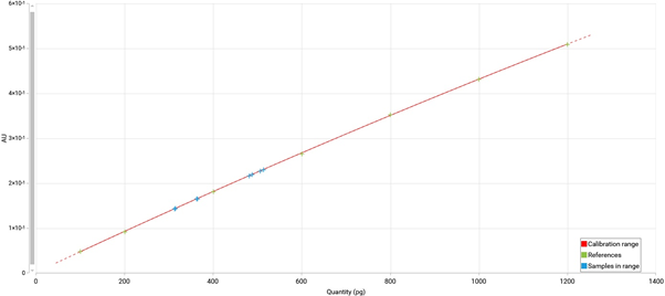
Example of an exported calibration curve (white background for all exported graphs)

Spectrum Scan

After single- or multi-wavelength scan, spectra of selected peaks can be recorded. For this, another scanner step is added.

In the Scanner settings the range can be selected, e.g. from 190 to 400 nm.

There are two options available: the classical spectrum scan of selected peaks or spectrum scan for purity testing. Purity testing is selected by a tick.

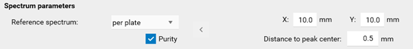
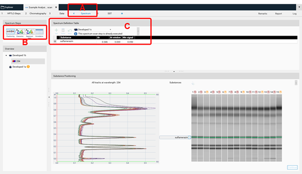
In this case for each peak a spectrum will be recorded at 3 positions comparing beginning, middle, and end of a peak (peak pure or co-elution of a compound). By clicking Continue in the Chromatography tab (to start the scanner step for spectrum scan) the Spectrum tab (A) is opened. visionCATS will guide you through all required steps (B). First the substance(s) and peaks are selected for spectrum scan (C).

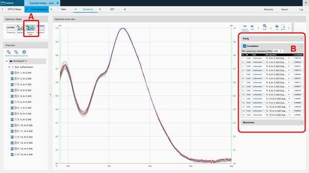
Then spectra will be recorded (Execution) and the data window opens (Spectrum data, (A)). At the rights side (B) the results (correlation) for either overlay of spectra obtained at the same RF on different tracks or overlay within one zone (start – middle – end) for purity testing are shown. Maxima can be displayed as well.

Working with Comparison files

Comparison files allow comparing sample tracks and/or spectra of substance peaks from the same and/or from different plates. This section uses the data of the “Comparison Viewer” demo file (download zip-folder at: Downloads) as an example.

Image Comparison

For Image Comparison select the tracks of interest from your analysis file (A), (B), (C). The tracks can be exported to an existing or a new Comparison file. By directly clicking (C) all tracks are selected for Comparison.

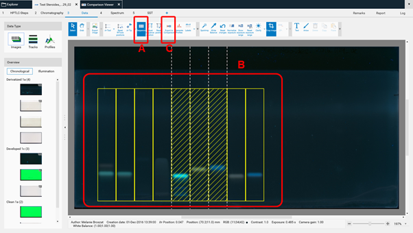
Clicking (C) opens a new window, asking for selecting the detection modes and steps for Comparison.

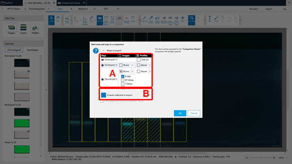
In (A) the steps of the captured images (e.g. before and after derivatization) and the detection modes (UV 254 nm, UV 366 nm, white light) can be selected. In (B) the tracks can be selected.

Then the selected tracks will be exported to an already open, existing Comparison file or the software will ask for the name of a new Comparison file. New tracks are added to the end (right side) of existing Comparison files. If several detection modes have been selected for Export to Comparison then (A) allows to switch between them.

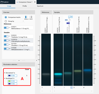
Switch within detection modes at (A)

Profile Comparison

For Profile Comparison tracks of interest are selected from the analysis file in the Data View tab (either Image tab or Profile tab). The tracks can be exported to an existing or a new Comparison file.

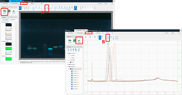
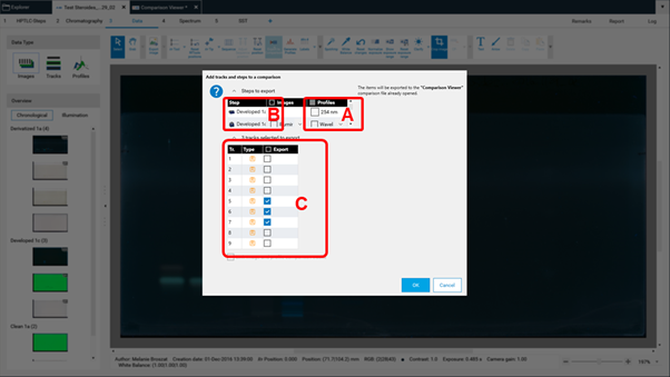
By clicking Export to Comparison a new window opens (see next image) asking for selecting the detection modes (A) and steps (B) for Comparison. In (C) the tracks can be selected.

The selected tracks for profile comparison will be exported to the open existing Comparison file or the software will ask for the name of the new Comparison file. New tracks are added to existing Comparison files at the end. There are different display modes: Overlay and Stack view.

Overlay view; Reference tracks can be moved up at (A) for Comparison.

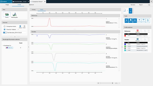
Stack view

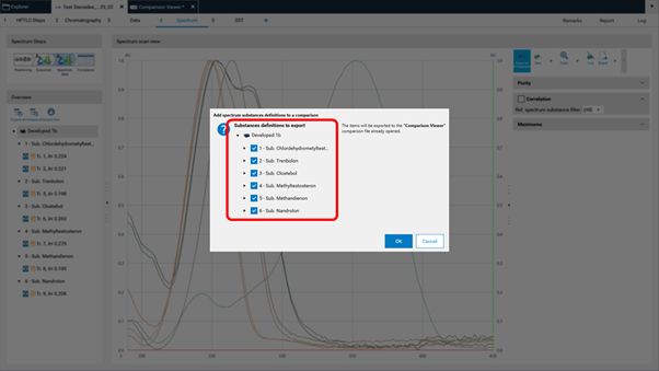
Spectrum Comparison

To compare spectra obtained from different substance zones click Export to Comparison (A) at the Spectrum data in the Spectrum tab of your analysis file.

A new window will open asking for selecting the substances (recorded spectra of substance zones) for Comparison.

Other features

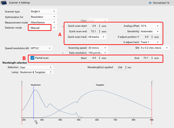
Quick scan / Partial scan

visionCATS allows a manual control of the TLC Scanner 3 and 4. Prior to the scanning densitometric measurement of all sample tracks, a quick scan is performed to adjust the photomultiplier (adjust offset of the detector). In certain cases, the sample matrix (especially in fluorescence detection mode) can have a larger signal response then the target. To focus on the target zone, the quick scan can be performed at a defined area of interest (on a single track, with a start and end position within the entire RF range) (A). Furthermore, a partial scan can be performed for scanning densitometric measurement of all sample tracks with defined start and end position within the entire RF range (B). This will lead to larger scaling of small peaks, needed for trace analysis.

Dual Wavelength scan and (blank) track subtraction

Background signals from matrices, solvent, etc. can cause problems during quantitative evaluation. In the Integration tab of the evaluation within the Expert mode, a Profile subtraction is available. Either a blank track (pure solvent applied) can be subtracted or in the case of a multi-wavelength scan, two scanned wavelengths can be subtracted (Dual wavelength).

AMD 2 settings

Chromatographic separation of complex samples is a challenging task for every laboratory, particularly when the components span a wide polarity range. The AMD (Automated Multiple Development) offers a convenient and most efficient solution. It employs stepwise elution over increasing solvent migration distances with a gradient that can be designed according to the requirements of the sample.

The principle

• Multiple development over increasing solvent migration distances

• Each successive run uses a solvent of lower elution strength than the previous

• Between runs the layer is dried under vacuum

The result

• Extremely narrow bands due to gradient elution with simultaneous focusing effect

• Enhanced separation capacity with base line separation of up to 40 components over a separation distance of 80 mm

• Highest resolution that can be attained with a planar chromatography system

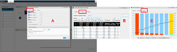
To perform a polarity gradient, an AMD step is added to the method template (HPTLC steps).

Then the parameters are entered in the Chromatography tab after selecting the instrument icon by a mouse click. In (A) the number of bottles is selected and the solvent are defined. In (B) the gradient is entered. In (C) a graph of the gradient can be seen.

Reports

Beginning with visionCATS version 2.4, custom report templates can be generated in addition to the provided templates. To change the content and design (global css) basic knowledge on html programming is required. Further information can be found in the visionCATS online help at Changing template styles.

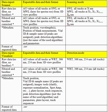
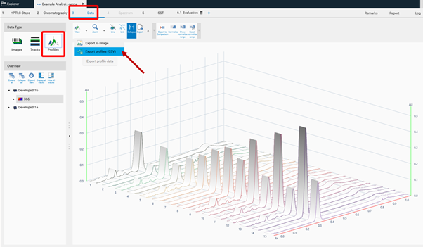
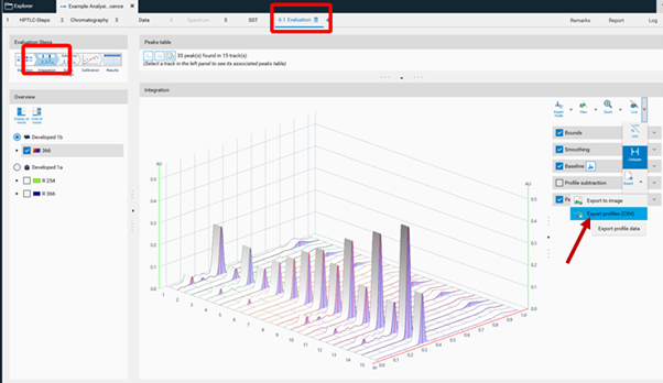
Export of Data

For visionCATS the option Export of Data can be purchased. This option allows exporting the raw data (all data points obtained by scanning densitometry or from captured images). There are two different ways for Export of Data with this option: raw data without filtering (smoothing algorithms) and baseline correction, and export of filtered and baseline corrected data. The data are exported as csv. files allowing an evaluation in Excel or MatLab, etc.

Export of Data

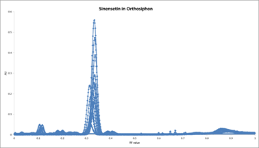
Example of a graph re-drawn in Excel

To get unmodified raw data, the csv. file is exported from the Data tab (Profiles).

To get filtered/baseline corrected data (use of peak detection algorithms, smoothing algorithms, etc.), the csv. file is exported from the Evaluation tab (Integration).

21 CFR Part 11

For visionCATS the option 21 CFR Part 11 can be purchased. This option includes: * System logger * E-Signature * options related to deletion * motivated change management

For further information, see 21CFR Part 11 compliance

Example Files

Several Example Analysis files can be downloaded at https://www.camag.com/downloads After importing the downloaded files to your own visionCATS database, making a copy is recommended. Imported files are in “read only” mode. No changes can be saved. Copied files can be used for training purposes.

Case studies with application tutorial videos

HPTLC-Fingerprint of Ginkgo biloba flavonoids (qualitative example)

https://www.camag.com/article/hptlc-fingerprint-ginkgo-biloba-flavonoids

Identification of fixed oils by HPTLC (qualitative example, including method transfer validation)

https://www.camag.com/article/identification-fixed-oils-hptlc

In-process control during chemical synthesis (qualitative example, including HPTLC-MS)

https://www.camag.com/article/process-control-during-chemical-synthesis-ergoline-psychedelics-hptlc

Quantitative determination of steviol glycosides (quantitative example)

https://www.camag.com/article/quantitative-determination-steviol-glycosides